exosim.utils.psf

Attributes

logger

Functions

create_psf(wl, fnum, delta[, nzero, shape, ...])

Calculates an Airy Point Spread Function arranged as a data-cube.

Module Contents

logger

create_psf(wl, fnum, delta, nzero=4, shape='airy', max_array_size=None, array_size=None)

Calculates an Airy Point Spread Function arranged as a data-cube. The spatial axes are 0 and 1. The wavelength axis is 2. Each PSF volume is normalised to unity.

Parameters:

• wl (Quantity) – array of wavelengths at which to calculate the PSF

• fnum (float or (float, float)) – Instrument f/number. It can be a tuple of two values, in which case the first value is the f/number for the x axis and the second value is the f/number for the y axis.

• delta (Quantity) – the increment to use [physical unit of length]

• nzero (float) – number of Airy zeros. The PSF kernel will be this big. Calculated at wl.max()

• shape (str (optional)) – Set to ‘airy’ for a Airy function,to ‘gauss’ for a Gaussian

• max_array_size ((int,int) (optional)) – Maximum size of the PSF array. If None, the size is calculated from the f/number and the wavelength range.

• array_size ((int or str,int or str) (optional)) – Size of the PSF array. If ‘full’ then the max_array_size are used. If None, the size is calculated from the f/number and the wavelength range.

Returns:

three-dimensional array. Each PSF normalised to unity

Return type:

ndarray

Examples

>>> import astropy.units as u
>>> from exosim.utils.psf import create_psf

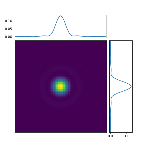
We produce and plot an Airy PSF:

>>> img = create_psf(1*u.um, 40, 6*u.um, nzero=8, shape='airy')

>>> import matplotlib.pyplot as plt
>>> import numpy as np
>>> from matplotlib.gridspec import GridSpec
>>> fig = plt.figure(figsize=(6, 6))
>>> gs = fig.add_gridspec(2, 2,  width_ratios=(4, 1), height_ratios=(1, 4),
>>>                       left=0.1, right=0.9, bottom=0.1, top=0.9,
>>>                       wspace=0.05, hspace=0.05)
>>> ax = fig.add_subplot(gs[1, 0])
>>> ax.imshow(img)
>>> ax_x = fig.add_subplot(gs[0, 0], sharex=ax)
>>> ax_y = fig.add_subplot(gs[1, 1], sharey=ax)
>>> axis_x = np.arange(0, img.shape[1])
>>> ax_x.plot(axis_x, img.sum(axis=0))
>>> ax_x.set_xticks([], [])
>>> axis_y = np.arange(0, img.shape[0])
>>> ax_y.plot(img.sum(axis=1), axis_y)
>>> ax_y.set_yticks([], [])
>>> plt.show()

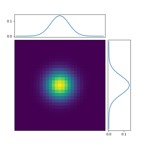
Similarly, we can produce and plot a Gaussian PSF:

>>> img = create_psf(1*u.um, (40,40), 6*u.um, shape='gauss')

>>> import matplotlib.pyplot as plt
>>> import numpy as np
>>> from matplotlib.gridspec import GridSpec
>>> fig = plt.figure(figsize=(6, 6))
>>> gs = fig.add_gridspec(2, 2,  width_ratios=(4, 1), height_ratios=(1, 4),
>>>                       left=0.1, right=0.9, bottom=0.1, top=0.9,
>>>                       wspace=0.05, hspace=0.05)
>>> ax = fig.add_subplot(gs[1, 0])
>>> ax.imshow(img)
>>> ax_x = fig.add_subplot(gs[0, 0], sharex=ax)
>>> ax_y = fig.add_subplot(gs[1, 1], sharey=ax)
>>> axis_x = np.arange(0, img.shape[1])
>>> ax_x.plot(axis_x, img.sum(axis=0))
>>> ax_x.set_xticks([], [])
>>> axis_y = np.arange(0, img.shape[0])
>>> ax_y.plot(img.sum(axis=1), axis_y)
>>> ax_y.set_yticks([], [])
>>> plt.show()

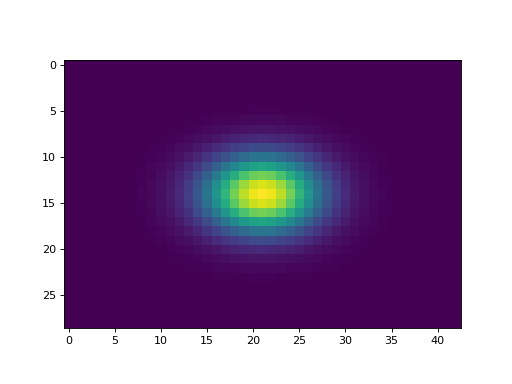
We can also create a PSF with different F-numbers:

>>> img = create_psf(1*u.um, (60,40), 6*u.um, shape='gauss')

>>> import matplotlib.pyplot as plt
>>> plt.imshow(img, aspect='equal',)
>>> plt.show()