Signals

The data flow in the code is handled by the exosim.models.signal.Signal class. Signals are similar to array but with methods and a math specifically designed for the code goal.

To understand better how they work, let’s produce a simple case:

import numpy as np
from exosim.models.signal import Signal

wl = np.linspace(0.1, 1, 10) * u.um
data = np.ones((10, 1, 10))
time_grid = np.linspace(1, 5, 10) * u.hr

signal = Signal(spectral=wl, data=data, time=time_grid)

The resulting signal variable now contains a Signal class. We can access the data stored in the data attribute. If units are attached to the data, are stored in the data_units.

The data are stored in a cube as described in the picture.

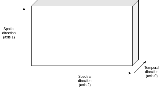
The grid used for the spectral direction (axis 2) is stored in the spectral attribute, with its units in spectral_units. Similarly, the grid used for the spatial direction (axis 1), if any, is stored in the spatial attribute, with its units in spatial_units, and the temporal grid (axis 0), if any, is stored in time with its units in time_units. If no information are provided for these grid the defaults values are \(0 \, \mu m\) for spectral and spatial axes and \(0 \, hr\) for temporal.

Also, metadata can be attach to a Signal class in the form a dictionary.

data = np.ones((10, 1, 10))
metadata = {'test': True}
signal = Signal(data=data, metadata=metadata)

or they can be attached later as

data = np.ones((10, 1, 10))
signal = Signal(data=data)
metadata = {'test': True}
signal.metadata = metadata

In both cases

>>> print(signal.metadata)
{'test': True}

Units

If any units is attached to the input data as in

data = np.ones(10)*u.m
signal = Signal(data=data)

Or they can be specified as:

data = np.ones(10)
signal = Signal(data=data, data_units=u.m)

Then, the data can be converted into a different units as

signal.to(u.cm)

Derived classes

Thanks to the units support, we can derive different derived classes:

• exosim.models.signal.Sed, which has units of \(W \, m^{-2} \, \mu m^{-1}\)

• exosim.models.signal.Radiance, which has units of \(W \, m^{-2} \, \mu m^{-1} \, sr^{-1}\)

• exosim.models.signal.CountsPerSecond, which has units of \(counts \, s^{-1}\)

• exosim.models.signal.Counts, which has units of \(counts\)

• exosim.models.signal.Adu, which has units of \(adu\)

• exosim.models.signal.Dimensionless, which has no units

The user can directly initialise one of these classes to specify the data units. Otherwise, if units are attached to the data, the main Signal class automatically detects the right derived class to use.

Mathematical operations

A set of mathematical operations is possible with the Signal class and it derived classes. Later here are listed the simplest examples to show the concept, however, the supported operation include:

• operations between Signal classes (as in the exaples);

• operations between a Signal and a numpy.ndarray or a Quantity;

• operations in reversed order (array + Signal instead of only Signal + array)

Also, the units are taken into account during the operation. In fact, multiplying a Dimensionless for a Sed results in a Sed, as multiply a exosim.models.signal.Radiance by a solid angle results in a Sed. It’s not possible to sum or subtract a Sed class to a Dimensionless. This, again, is true not only between Signal classes, but also when operating Signal classes and Quantity.

Finally the operations involving Signal classes also work on cached classes. See Cached signals for more.

Sum

import numpy as np
import astropy.units as u
from exosim.models.signal import Signal

data = np.ones((3))
signal1 = Signal(data=data)

data = np.ones((3)) * 2
signal2 = Signal(data=data)

signal3 = signal1 + signal2

and hence

>>> print(signal3.data)
[[[3. 3. 3.]]]

Subtraction

import numpy as np
import astropy.units as u
from exosim.models.signal import Signal

data = np.ones((3))
signal1 = Signal(data=data)

data = np.ones((3)) * 2
signal2 = Signal(data=data)

signal3 = signal1 - signal2

and hence

>>> print(signal3.data)
[[[-1. -1. -1.]]]

Multiplication

import numpy as np
import astropy.units as u
from exosim.models.signal import Signal

data = np.ones((3))
signal1 = Signal(data=data)

data = np.ones((3)) * 2
signal2 = Signal(data=data)

signal3 = signal1 * signal2

and hence

>>> print(signal3.data)
[[[2. 2. 2.]]]

Division

import numpy as np
import astropy.units as u
from exosim.models.signal import Signal

data = np.ones((3))
signal1 = Signal(data=data)

data = np.ones((3)) * 2
signal2 = Signal(data=data)

signal3 = signal1 / signal2

and hence

>>> print(signal3.data)
[[[0.5 0.5 0.5]]]

Floor division

import numpy as np
import astropy.units as u
from exosim.models.signal import Signal

data = np.ones((3))
signal1 = Signal(data=data)

data = np.ones((3)) * 2
signal2 = Signal(data=data)

signal3 = signal1 // signal2

and hence

>>> print(signal3.data)
[[[0. 0. 0.]]]

Binning operation

Among the useful methods included in the exosim.models.signal.Signal class, it is worth mentioning the binning. There are two binning methods included in the class:

• exosim.models.signal.Signal.spectral_rebin to rebing the dataset in the spectral direction

• exosim.models.signal.Signal.temporal_rebin to rebing the dataset in the time direction

They are both based on exosim.utils.binning.rebin. The function resamples a function fp(xp) over the new grid x, rebinning if necessary, otherwise interpolates, but it does not perform extrapolation. The function is optimised to resample multidimensional array along a given axis.

Both spectral_rebin and temporal_rebin are described with examples in their documentation. Let’s use as example here the case of a spectral binning. We first define the initial values:

>>> wavelength = np.linspace(0.1, 1, 10) * u.um
>>> data = np.ones((10, 1, 10))
>>> time_grid = np.linspace(1, 5, 10) * u.hr
>>> signal = Signal(spectral=wavelength, data=data, time=time_grid)
>>> print(signal.data.shape)
(10,1,10)

We can interpolates at a finer wavelength grid:

>>> new_wl = np.linspace(0.1, 1, 20) * u.um
>>> signal.spectral_rebin(new_wl)
>>> print(signal.data.shape)
(10,1,20)

or we can bin down the to a new wavelength grid:

>>> signal = Signal(spectral=wavelength, data=data, time=time_grid)
>>> new_wl = np.linspace(0.1, 1, 5) * u.um
>>> signal.spectral_rebin(new_wl)
>>> print(signal.data.shape)
(10,1,5)

Writing, copying and converting

Other useful methods are related to the capability to export the information content of a exosim.models.signal.Signal class.

A exosim.models.signal.Signal can be casted into a dict object as

import numpy as np
from exosim.models.signal import Signal

data = np.ones((3))
signal = Signal(data=data)

dict(signal)

This will result in a dictionary with keys named after the class attributes with their content as value. The casting operation only conserves some of the exosim.models.signal.Signal class information. The attributes that are casted are: data, time, spectral, spatial, metadata, data_units, time_units, spectral_units, and spatial_units.

>>> print(dict(signal))
{'data': array([[[1., 1., 1.]]]),
 'time': array([0.]),
 'spectral': array([0.]),
 'spatial': array([0.]),
 'metadata': {},
 'data_units': '',
 'time_units': 'h',
 'spectral_units': 'um',
 'spatial_units': 'um'}

The exosim.models.signal.Signal.write method allow to store the content into and Output class. More commonly, into an HDF5 file. In the following example, we show how to store the signal class into an output file.

import os
from exosim.output.hdf5.hdf5 import HDF5Output

output = os.path.join("output_test.h5")
with HDF5Output(output) as o:
    signal.write(o, "test_signal")

Then, the output will contains the class information as:

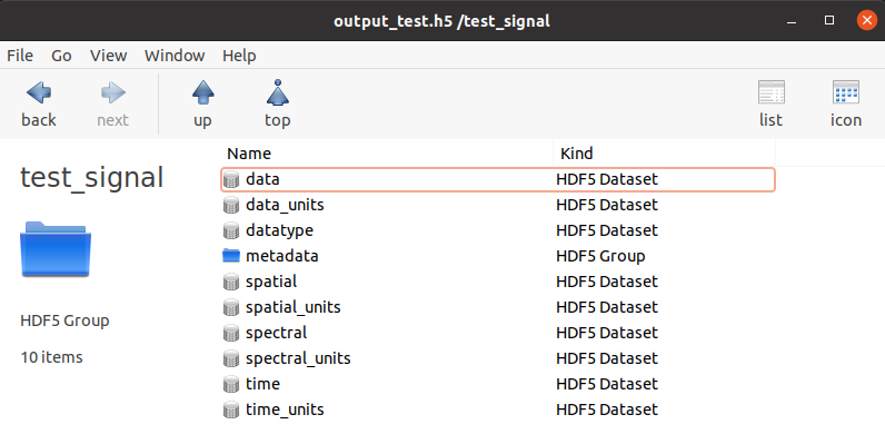
The information stored are the same of dict(signal)

Also, an iterator has been implemented in the Signal class, such that the user can access the information as

>>> for k,v in signal1: print(k,v)
data [[[1. 1. 1.]]]
time [0.]
spectral [0.]
spatial [0.]
metadata {}
data_units
time_units h
spectral_units um
spatial_units um

Finally, a Signal class can be copied to a new class, thanks to the exosim.models.signal.Signal.copy method:

copied_signal = signal.copy()

Cached signals

Signal classes can be used in cached mode to handle huge datasets. This is enabled by chucked h5py.Dataset. The Signal are supported by the The CachedData class. To produce a cached Signal the user must indicate a HDF5OutputGroup or HDF5Output, the data set shape, and a dataset name:

import numpy as np
import astropy.units as u

from exosim.models.signal import Signal
from exosim.output import SetOutput

output = SetOutput('test_file.h5')
with output.use(append=True, cache=True) as out:
    cached_signal = Signal(spectral = np.arange(0,100) * u.um,
                            data=None,
                            shape=(1000,100,100),
                            cached=True, output=out,
                            dataset_name='cached_dataset')

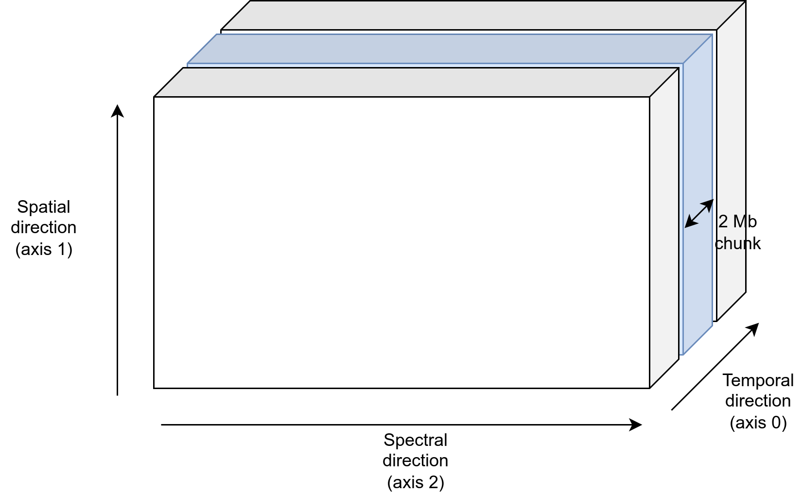
The dataset is stored in the indicated file un chunks of the user-defined size. By default the chunk size is set to 2 MB. Each chunk is a cube of the full spectral and spatial shapes and the number of time steps needed to weigh 2 MB.

Then, the chunk size can be set using the RunConfig class, as described in Chunk size:

from exosim.utils import RunConfig

RunConfig.chunk_size = N

where N is the desired size of chunk in MB, which will be set for the environment.

If no output file is indicated, the code produce a temporary file. Having a cached Signal is little different from a normal one. While for the normal one we usually access the datacube content using the data attribute, for a cached Signal is preferred to use the dataset: while the former forces the system to load all the datacube, which should be avoided for big dataset, the latter refers to the associate chunked h5py.Dataset class.

To access the chunks and set the dataset values, one can use the h5py.Dataset methods. In the following example, we iterate over the class chunks and set the values to 1.

for chunk in cached_signal.dataset.iter_chunks():
    dset = np.ones(cached_signal.dataset[chunk].shape)
    cached_signal.dataset[chunk] = dset

Otherwise, the data can be accessed as a normal numpy array

cached_signal.dataset[10,10,10] = 1

Note

A cached Signal allows the access to the associated h5py.Dataset only as long as the HDF5Output is open.

To be sure to apply the edit to the dataset in the open file, remember to flush them:

cached_signal.output.flush()

Finally, if the user wants to loop over the chunks, a dedicate util is available in ExoSim: iterate_over_chunks

for chunk in iterate_over_chunks(cached_signal.dataset,
                             desc="iterator description"):
    dset = np.ones(cached_signal.dataset[chunk].shape)
    cached_signal.dataset[chunk] = dset
    cached_signal.output.flush()