Sources#
Inputs: describe the source#
The target source must be described in an .xml file under sky, using the keyword source.
In the following example we simulate HD 209458:
<source> HD 209458
<source>
This file will be parsed by LoadOptions into a dictionary,
and the star name is stored under the keyword value.
loadOptions = LoadOptions()
options = loadOptions(filename = 'path/to/file.xml')
options['value'] = 'HD 209458'
The dictionary is then feeded to the ParseSource task, that returs the source Sed.
ExoSim supports three different sources type:
The source type is to be indicated as:
<source> HD 209458
    <source_type> planck </source_type>
</source>
According to the indicated type, ParseSource will call a different Task.
Planck star#
If planck star is used, then other information are needed to simulate the source:
<source> HD 209458
    <source_type> planck </source_type>
    <R unit="R_sun"> 1.18 </R>
    <T unit="K"> 6086 </T>
    <D unit="pc"> 47 </D>
</source>
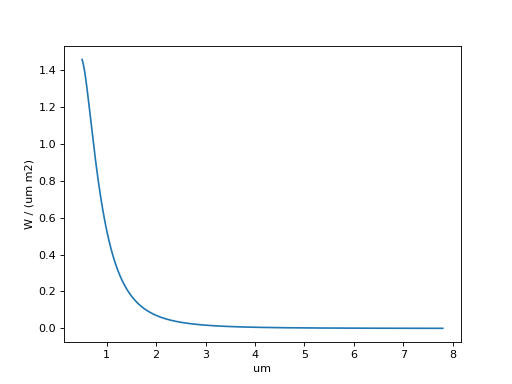
The planck star sed is created by CreatePlanckStar:
The star emission is simulated by astropy.modeling.physical_models.BlackBody.
The resulting sed is then converted into \(W/m^2/sr/\mu m\) and scaled by the solid angle \(\pi \left( \frac{R}{D} \right)^2\).
Here we report and example:
from exosim.tasks.sed import CreatePlanckStar
import astropy.units as u
import numpy as np
createPlanckStar = CreatePlanckStar()
wl = np.linspace(0.5, 7.8, 10000) * u.um
T = 6086 * u.K
R = 1.18 * u.R_sun
D = 47 * u.au
sed = createPlanckStar(wavelength=wl, T=T, R=R, D=D)

import matplotlib.pyplot as plt
plt.plot(sed.spectral, sed.data[0,0])
plt.ylabel(sed.data_units)
plt.xlabel(sed.spectral_units)
plt.show()
Phoenix star#
If phoenix is indicated, then ExoSim uses the Phoenix spectral irradiances to simulate the source. In this case we can either point to a specific Phoenix file using the filename keyword:
<source> HD 209458
    <source_type>phoenix </source_type>
    <filename> phoenix_filename </filename>

    <R unit="R_sun"> 1.18 </R>
    <D unit="pc"> 47 </D>
</source>
or we can point ExoSim to a path containing all the Phoenix spectra and provide it with all the information to select the best spectra to use:
<source> HD 209458
    <source_type>phoenix </source_type>
    <path> phoenix_path </path>

    <R unit="R_sun"> 1.18 </R>
    <M unit="M_sun"> 1.17 </M>
    <T unit="K"> 6086 </T>
    <D unit="pc"> 47 </D>
    <z unit=""> 0.0 </z>
</source>
The Phoenix star sed is created by LoadPhoenix: the Phoenix sed has units of \(W/m^2/\mu m\) and is scaled by \(\left( \frac{R}{D} \right)^2\).
Custom star#
If custom is indicated, then ExoSim will either look for a custom Task (see Custom Tasks), if source_task is present in the configuration file, or by default it uses LoadCustom.
The Task loads a custom SED from a file and scaled it by the solid angle \(\pi \left( \frac{R}{D} \right)^2\).
The default LoadCustom needs a filename containing the Sed to use.
<source> HD 209458
    <source_type>custom </source_type>
    <filename> custom_sed_filename </filename>

    <R unit="R_sun"> 1.18 </R>
    <D unit="pc"> 47 </D>
</source>
The custom sed file must be a .ecsv file with two columns: Wavelength and Sed, where the sed has units of \(W/m^2/sr/\mu m\).
Note
Depending on the computing power available, the user can decide to use a different number of wavelength and temporal points to simulate the source, incrementing the simulation accuracy.
Note
Spectral Irradiance vs. Spectral Radiance
The distinction between Phoenix SEDs and the Planck/Custom SEDs lies in their physical definition:
Phoenix SEDs represent spectral irradiance, with units of \(W/m^2/\mu m\). They describe the flux received per unit area at a given distance.
Planck and Custom SEDs represent spectral radiance, with units of \(W/m^2/sr/\mu m\). These include the angular distribution of emitted radiation.
To ensure consistency, ExoSim applies a scaling factor of \(\left( \frac{R}{D} \right)^2\) to all SEDs. However, only Planck and Custom SEDs include an additional factor of \(\pi\), accounting for the assumption of isotropic emission over a hemisphere.
Load star parameters from online databases#
ExoSim can load star parameters from online databases. At the moment only exodb is supported.
In this case, instead of the stellar parameter, the online database must be indicated:
<source> HD 209458
    <source_type>phoenix </source_type>
    <path>/usr/local/project_data/sed </path>

    <online_database>
        <url>https://exodb.space/api/v1/star</url>
        <x-access-tokens> your_token_here </x-access-tokens>
    </online_database>

</source>
Create your own source#
Otherwise, in Exosim you can create your own source by using a customizable Task.
To learn more about customizing tasks, please refer to Custom Tasks.
To create a custom source, use CreateCustomSource.
As an example, we report here the default CreateCustomSource task.
To enable it, write the following in your xml file:
<source> HD 209458
    <source_task> CreateCustomSource </source_task>
    <R unit="R_sun"> 1.17967 </R>
    <T unit="K"> 6086 </T>
    <D unit="pc"> 47.4567 </D>
    <wl_min unit="um">0.5</wl_min>
    <wl_max unit="um">8</wl_max>
    <n_points >1000</n_points>
</source>
The source_task keyword will guide the code to the Task to use. In this case is the default tasks.
If you write your own version, please write there the file containing your script.
The default CreateCustomSource task will simply create a planck star using the input parameters.
Outputs: prepare the sources#
Single source#
As mentioned, the .xml file parsed by LoadOptions,
for the planck case it will return a dictionary similar to
source_in = {
        'value': 'HD 209458',
        'source_type': 'planck',
        'R': 1.18 * u.R_sun,
        'D': 47 * u.pc,
        'T': 6086 * u.K,
        }
The wavelength grid to use is provided by the Wavelength grid.
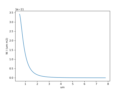
Then, we can use ParseSource task to produce the Sed.
The result will be a dictionary with the star name as keys and Sed as key content.
from exosim.tasks.parse import ParseSource
import astropy.units as u
import numpy as np
parseSource = ParseSource()
wl = np.linspace(0.5, 7.8, 10000) * u.um
tt = np.linspace(0.5, 1, 10) * u.hr

source_out = parseSource(parameters=source_in,
                         wavelength=wl,
                         time=tt)

import matplotlib.pyplot as plt

plt.plot(source_out['HD 209458'].spectral, source_out['HD 209458'].data[0,0])
plt.ylabel(source_out['HD 209458'].data_units)
plt.xlabel(source_out['HD 209458'].spectral_units)
plt.show()
More sources#
If more sources are listed, the xml file will look like this:
<source> HD 209458
    <source_type> planck </source_type>
    <R unit="R_sun"> 1.18 </R>
    <T unit="K"> 6086 </T>
    <D unit="pc"> 47 </D>
</source>

<source> GJ 1214
    <source_type> planck </source_type>
    <R unit="R_sun"> 0.218 </R>
    <T unit="K"> 3026 </T>
    <D unit="pc"> 13 </D>
</source>
Then, the parsed dictionary will be:
from collections import OrderedDict
sources_in = OrderedDict({'HD 209458': {'value': 'HD 209458',
                                    'source_type': 'planck',
                                    'R': 1.18 * u.R_sun,
                                    'D': 47 * u.pc,
                                    'T': 6086 * u.K,
                                    },
                            'GJ 1214': {'value': 'GJ 1214',
                                    'source_type': 'planck',
                                    'R': 0.218 * u.R_sun,
                                    'D': 13 * u.pc,
                                    'T': 3026 * u.K,
                                    },})
And this dictionary is fed into ParseSources to produce the following Sed:
import astropy.units as u
import numpy as np
from exosim.tasks.parse import ParseSources

wl = np.linspace(0.5, 7.8, 10000) * u.um
tt = np.linspace(0.5, 1, 10) * u.hr

parseSources = ParseSources()
sources_out = parseSources(parameters=sources_in,
                           wavelength=wl,
                           time=tt)

import matplotlib.pyplot as plt

for key in sources_out.keys():
    plt.plot(sources_out[key].spectral, sources_out[key].data[0, 0], label=key)
plt.ylabel(sources_out[key].data_units)
plt.xlabel(sources_out[key].spectral_units)
plt.legend()
plt.show()
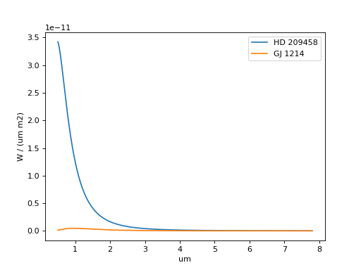
Note
In this example the sources are superimposed. If the sources have different position in the sky, see Telescope pointing and multiple sources. In that section is explained how to simulate multiple sources and the telescope pointing.
Parse from xml#
Assuming the wavelength and temporal grids have already produced as described in Wavelength grid and Temporal grid, you can parse the configuration file to produce a dictionary of sources as
import exosim.tasks.parse as parse

with output.use(append=True, cache=True) as out:

    out_sky = out.create_group('sky')

    parseSources = parse.ParseSources()
    sources = parseSources(parameters=mainConfig['sky']['source'],
                           wavelength=wl_grid,
                           time=time_grid,
                           output=out_sky)
Here we also assumed that the user selected an output file (as described in Preparing output) and wants to store the products in a dedicated subfolder.