Finalising the Sub-Exposures

Add background sub-exposures

Because more sources can be in the field of view (see Multiple sources in the field), ExoSim allows to include the background in the sub-exposures. The background stars are read using the same procedure described in Instantaneous readout, with the same readout parameters used for the target star.

The resulting sub-exposures are added to the focal plane sub-exposures, and stored back in the output.

To include the background to the produced sub-exposures just enable it on the configuration file, setting the option to True.

<channel> channel_name
    <detector>
        <add_background_to_se> True </add_background_to_se>
    </detector>
</channel>

Add foregrounds sub-exposures

Similarly to what has been done for the focal planes, once the sub-exposure are completed, we operate on the diffused light foregrounds.

To include the foregrounds to the produced sub-exposures just enable it on the configuration file, setting the option to True.

<channel> channel_name
    <detector>
        <add_foregrounds_to_se> True </add_foregrounds_to_se>
    </detector>
</channel>

If the keyword is missing, the foregrounds are included by default.

For each of the sub-exposures in the output we select the foreground focal plane corresponding to the acquisition time, and we multiplied it by the integration time. The resulting foreground sub-exposure is added to the focal plane sub-exposure and stored back in the output.

This is handled by AddForegrounds task.

import exosim.tasks.subexposures as subexposures

addForegrounds = subexposures.AddForegrounds()
se_out = addForegrounds(subexposures=se_out, frg_focal_plane=frg_fp,
                        integration_time=integration_times)

With clear reference to the quantities defined above.

Resulting sub-exposure

The resulting sub-exposures will look similar to the followings:

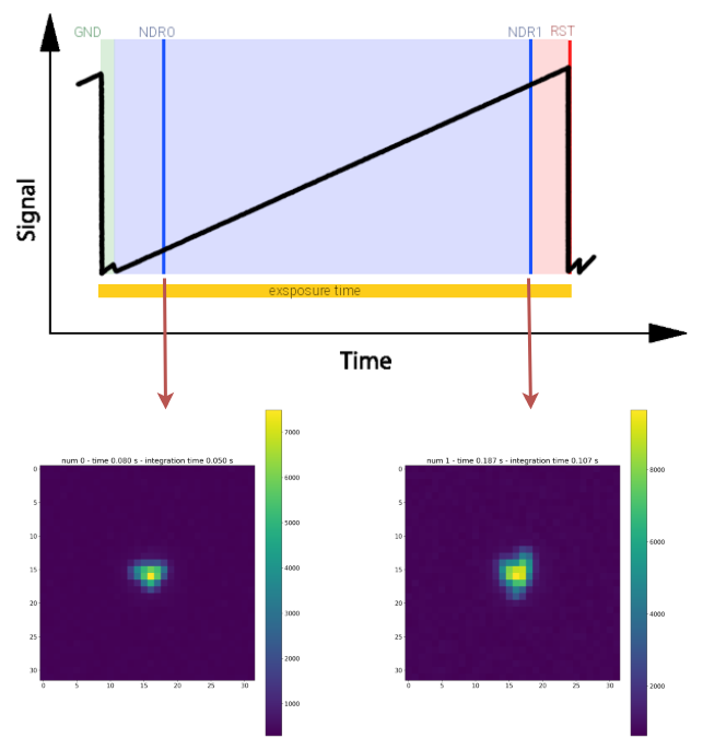
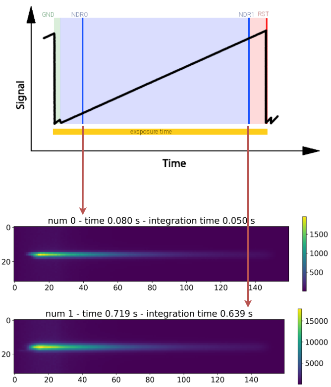
These examples have been produced with the procedure described in Sub-Exposures Plotter.

Quantum efficiency variation

Each pixel in the focal plane has a slightly different Quantum Efficiency (QE) from the others. This behaviour can be simulated in ExoSim by editing the normalisation of the pixel QEs

This can be set with a custom Task, as described in Custom Tasks, or by using the default LoadQeMap task. This task loads the QE variation map pre-computed from and .h5 file. If the user has its own map, can write a custom task load this map into a Signal class. Otherwise, ExoSim includes a tool (ExoSim Tools) which allow the creation of a quantum efficiency variation map (see Quantum efficiency variation map), which can be stored and used in successive simulations.

The Task to use to laod the QE variation map should be indicated under the channel detector configuration using the qe_map_task keyword. In the following we report the example using the default LoadQeMap task:

<channel> channel_name
    <detector>
        <qe_map_task> LoadQeMap </qe_map_task>
        <qe_map_filename> __ConfigPath__/data/payload/qe_map.h5 </qe_map_filename>
    </detector>
</channel>

where the qe_map_filename keyword indicates the quantum efficiency variation map to use for every channel of the payload.

Alternatively, the map can be provided as a simple numpy array (see numpy documentation) and parsed by the LoadQeMapNumpy task:

<channel> channel_name
    <detector>
        <qe_map_task> LoadQeMapNumpy </qe_map_task>
        <qe_map_filename> qe_map.npy </qe_map_filename>
    </detector>
</channel>

The resulting map is then applied to all the focal planes in the channel by the ApplyQeMap tasks. Because the quantum efficiency variation map can be time dependent, but sampled at a different cadence than the Sub-Exposure, in the Sub-Exposure signal is included a new key in the metadata: qe_variation_map_index. This array contains the indexes of the quantum efficiency realisation used for each of the sub-exposure: the array is as long as the sub-exposure temporal axis, and for each time step is reported the time index of the quantum efficiency variation map applied to that sub-exposure.

If no quantum efficiency variation map is provide, the code skip this step raising a Warning.