exosim.utils.binning

Attributes

logger

Functions

rebin(x, xp, fp[, axis, mode, fill_value])

This function can resample multidimensional array along a given axis.

Module Contents

rebin(x, xp, fp, axis=0, mode='mean', fill_value=0.0)

This function can resample multidimensional array along a given axis. Resample a function fp(xp) over the new grid x, rebinning if necessary, otherwise interpolates. Interpolation is done using ‘linear’ method. This function doesn’t perform extrapolation: unsample coordinates will be filled with filled value.

Parameters:

• x (ndarray) – New coordinates

• fp (ndarray) – y-coordinates to be resampled

• xp (ndarray) – x-coordinates at which fp are sampled

• axis (int (optional)) – fp axis to resample. Default is 0.

• mode (str (optional)) – the mode indicates the statistc to use for binning by scipy.stats.binned_statistic. Default is ‘mean’.

• fill_value (float or str (optional)) – fill value for unsampled coordinates. Default is 0.0.

Returns:

re-sampled fp

Return type:

ndarray

Raises:

NotImplementedError – If the mode is not implemented.

Examples

>>> import numpy as np
>>> from exosim.utils.binning import rebin

We define the original function, sampled in data 50 points:

>>> xp = np.linspace(1,10, 50)
>>> fp = np.sin(xp)

We bin it down, sampling it at 10 points

>>> x_bin = np.linspace(1,10, 10)
>>> f_bin = rebin(x_bin, xp, fp)

We wl_interpolate the original function, sampling it at 100 points

>>> x_inter = np.linspace(1,10, 100)
>>> f_inter = rebin(x_inter, xp, fp)

To compare the outcome of our interpolation, we produce a plot.

>>> import matplotlib.pyplot as plt
>>> fig, (ax0, ax1) = plt.subplots(2,1)

In the top panel we want to see the original function compared to the binned one and the interpolated one.

>>> ax0.plot(xp, fp, label='original array', alpha=0.5, c='r')
>>> ax0.scatter(x_inter, f_inter, marker='X', label='interpolated array', alpha=0.5)
>>> ax0.scatter(x_bin, f_bin, marker='V', label='binned array', alpha=0.5)
>>> ax0.legend()

In the bottom panel we compare each function with the true value and we divide this quantity by the true value.

>>> ax1.axhline(0, c='r', alpha=0.5)
>>> ax1.scatter(x_inter, (f_inter- np.sin(x_inter))/np.sin(x_inter),
...             marker='X', label='interpolated array', alpha=0.5)
>>> ax1.scatter(x_bin, (f_bin - np.sin(x_bin))/np.sin(x_bin),
...             marker='v', label='binned array', alpha=0.5)
>>> ax1.legend()
>>> plt.show()

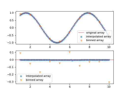
It’s important to notice here that when we perform the binning, we are not simply resampling the input function, but we are using the mean value inside each of the bins.

logger