Plotters

ExoSim 2 includes some plotters which allows a fast evaluation of the produced data. The default plotter can be run from console as exosim-plot.

The scipt includes two plotters: FocalPlanePlotter and RadiometricPlotter.

Focal plane Plotter

FocalPlanePlotter handles the methods to plot the focal planes produced by exosim.

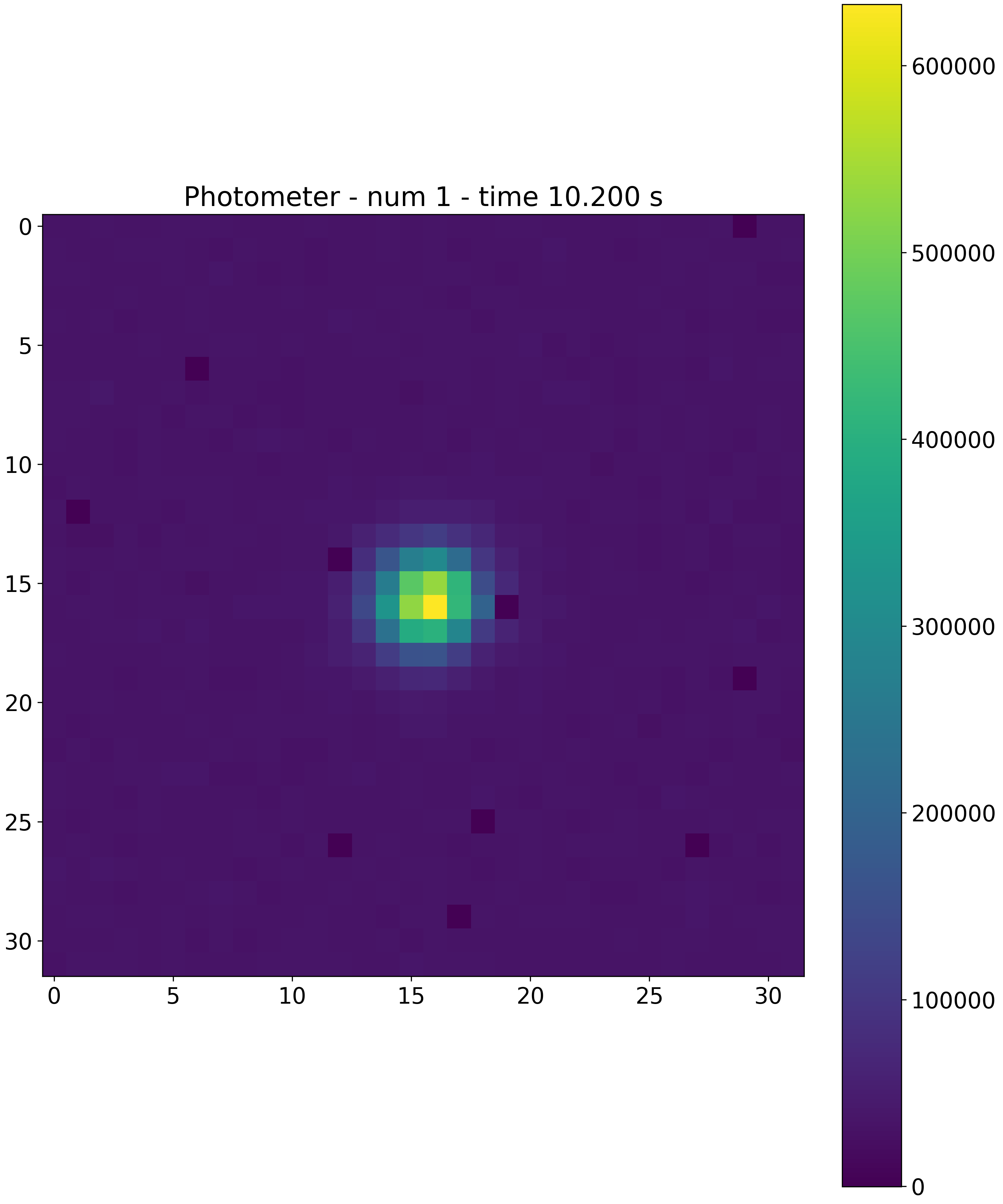
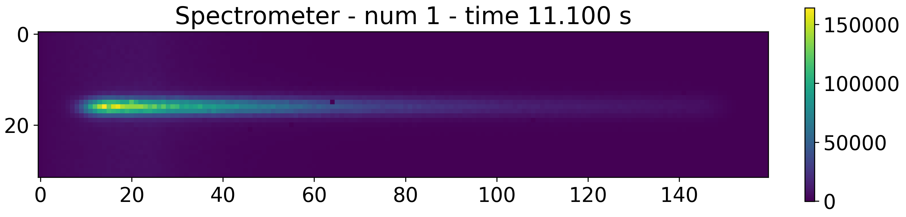
It plots the focal planes of each channel at a specific time. For each channel it adds a Axes to a figure. It returns a Figure with two rows: on the first row are reported the oversampled focal planes. In the second row are reported the extracted focal plane, where the oversampling is removed. The focal plane plotted is the combination of the source focal plane plus the foreground focal plane.

Given the test_file.h5 produced by Exosim, to plot the focal plane at the first time step, the user can run from console

exosim-plot -i test_file.h5 -o plots/ -f -t 0 --plot-scale linear

where -o is the output directory, -f is to run the focal plane plotter (FocalPlanePlotter) and -t is to select the time step, --plot-scale indicate the image scale to use. By default the plot scale is linear, but another possible option is dB, and the image is plotted as \(10 \cdot log_{10} \left( ima/ max(ima) \right)\).

The result will be similar to

The same result can be obtained also by using the plotter in a python script:

from exosim.plots import FocalPlanePlotter
focalPlanePlotter = FocalPlanePlotter(input='./test_file.h5')
focalPlanePlotter.plot_focal_plane(time_step=0, scale='linear')
focalPlanePlotter.save_fig('focal_plane.png')

if -plot-scale is set to dB the result will be

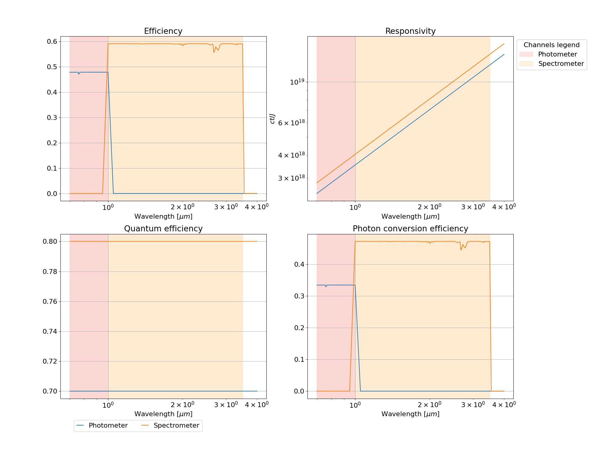
Inside the focal plane plotter a functionality to plot the total efficiency can be found:

from exosim.plots import FocalPlanePlotter
focalPlanePlotter = FocalPlanePlotter(input='./test_file.h5')
focalPlanePlotter.plot_efficiency()
focalPlanePlotter.save_fig('efficiency.png')

Radiometric Plotter

RadiometricPlotter handles the methods to plot the radiometric table produced by exosim.

Given the test_file.h5 produced by Exosim and which includes a radiometric table, to plot the table the user can run from console

exosim-plot -i test_file.h5 -o plots/ -r

where -o is the output directory and -r is to run the radiometric plotter (RadiometricPlotter).

The result will be similar to

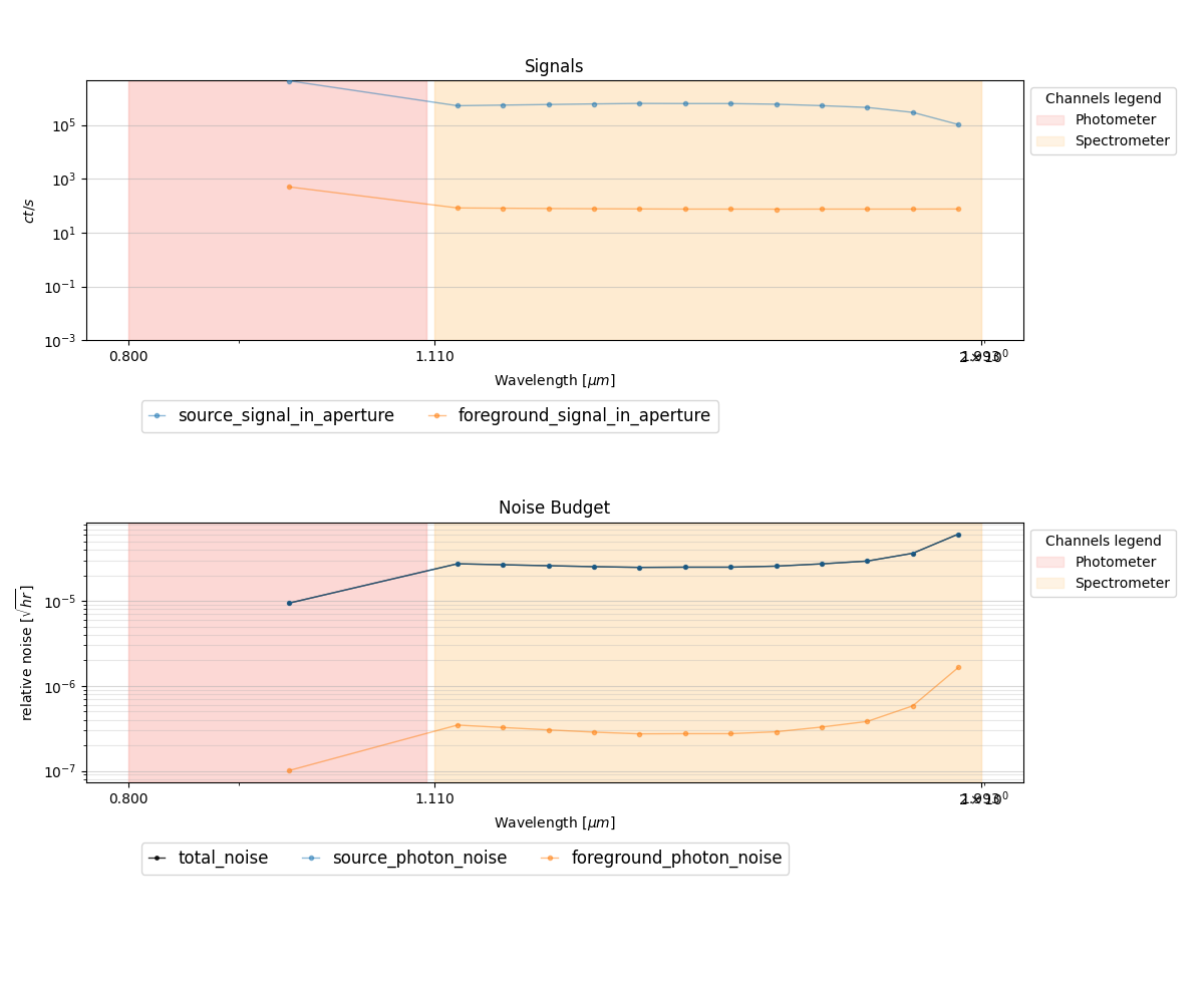
The same result can be obtained also by using the plotter in a python script:

from exosim.plots import RadiometricPlotter
radiometricPlotter = RadiometricPlotter(input='./test_file.h5')
radiometricPlotter.plot_table()
radiometricPlotter.save_fig('radiometric.png')

The radiometric plotter can also plot the apertures superimposed to the focal planes with

from exosim.plots import RadiometricPlotter
radiometricPlotter = RadiometricPlotter(input='./test_file.h5')
radiometricPlotter.plot_apertures()
radiometricPlotter.save_fig('apertures.png')

Sub-Exposures Plotter

SubExposuresPlotter handles the methods to plot the Sub-Exposures produced CreateSubExposures, as described in Sub-Exposures.

Given the test_se.h5 produced by ExoSim and which includes the sub-exposures, to plot them, the user can run from console

exosim-plot -i test_se.h5 -o plots/ --subexposures

or

exosim-plot -i test_se.h5 -o plots/ -s

SubExposuresPlotter iteratively store the images of the sub-exposures in the output folder, along with the sub-exposure time (which is the time where the sub-exposure integration ends) and the integration time.

Here we report for example the first and the second sub-exposures, collected using a CDS reading scheme, for both the channels

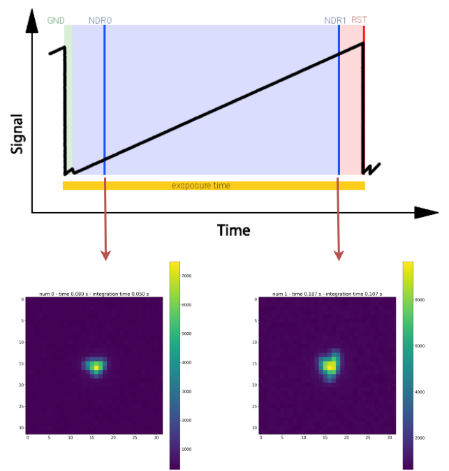
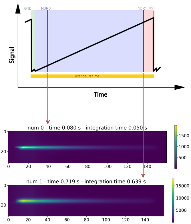
Note

Because the ExoSim output may contain a lot of sub-exposures, This plotter only produces images of the sub-exposures of the first exposure (the first ramp).

NDRs Plotter

NDRsPlotter handles the methods to plot the Sub-Exposures produced CreateNDRs, as described in NDRS.

Given the test_ndrs.h5 produced by ExoSim and which includes the NDRs, to plot them, the user can run from console

exosim-plot -i test_ndrs.h5 -o plots/ -ndrs

or

exosim-plot -i test_ndrs.h5 -o plots/ -n

NDRsPlotter iteratively stores the images of the NDRs in the output folder, along with the NDR exposure time.