Quick start#
In the following, we explore the main uses of the new ExoSim version. The code can be either used as stand-alone and run pre-made pipelines called recipes, or can be used as a library to build custom pipelines.
While in the next section of this documentation, we will focus on the functionalities contained in each recipe, and hence on the use of the code as a library, here we want to focus on the fast run.
Running ExoSim from console#
After the installation, the user can run ExoSim from the console to verify the installed version:
exosim
To run pre-made pipelines (called recipes’) the user can call exosim from the console after the installation.
Different recipes have different commands:
command |
description |
|---|---|
|
runs the recipe to create the low-frequency focal plane (Focal plane creation) |
|
runs the radiometric model recipe (Radiometric Model) |
|
create the sub-exposures from the focal plane (Sub-Exposures) |
|
create the ndrs from the sub-exposures (NDRS) |
Run it with the help flag to read the available options:
exosim-focalplane --help
Tip
The user can access the specific command also from the general exosim command by adding the specific command after it:
exosim focalplane --help
Here are listed the command line main flags.
flag |
description |
|---|---|
|
Input payload description file |
|
output file |
|
runs the associated plotter (Plotters) |
|
number of threads for parallel processing |
|
debug mode screen |
|
store the log output on file |
Where the configuration file shall be an .xml file and the output file and .h5 file (see later in The .h5 file) -n must be followed by an integer. -d and -l do not need any argument as they simply need to be listed to activate their options.
Understanding the outputs#
It’s easy.
The .h5 file#
The main output product is a HDF5 .h5 file. This format has many viewers such as HDFView or HDFCompass and APIs such as Cpp, FORTRAN and Python.
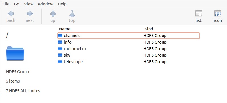
To use the data, see How can I load HDF5 data into my code? in the FAQs section.
Running the examples#
If you downloaded ExoSim 2 from the GitHub repository (see install git), you will find an examples folder in the root. If you installed ExoSim 2 from Pypi (see install pip), you will have to download the folder from the GitHub repository. Once you have downloaded the example folder, locate yourself there with the command console.
To run the example, you first need to change the path to the example folder in the main_example.xml file. Replace the path in the main_example.xml file with the path to the examples folder in your computer.
<ConfigPath>/path/to/ExoSim2/examples</ConfigPath>
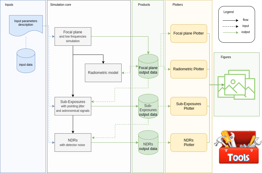
Now, we will follow the Exosim diagram
From console#
Focal plane#
The first step is to build the focal plane (see Focal plane creation). You can do it by
exosim-focalplane -c main_example.xml -o test_common.h5
Then you will find the output file in the same folder. If you want to produce the plots, you can now run
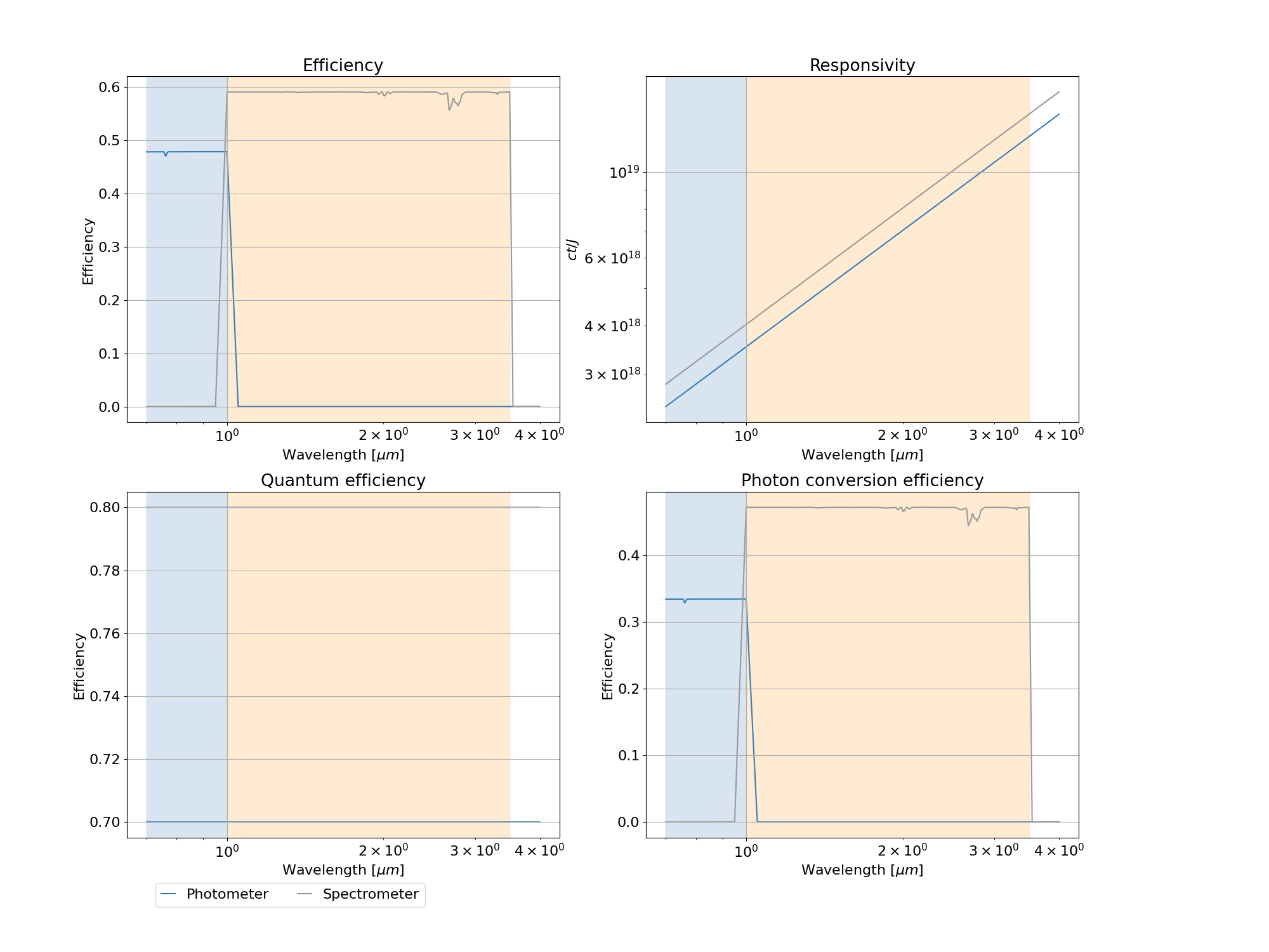
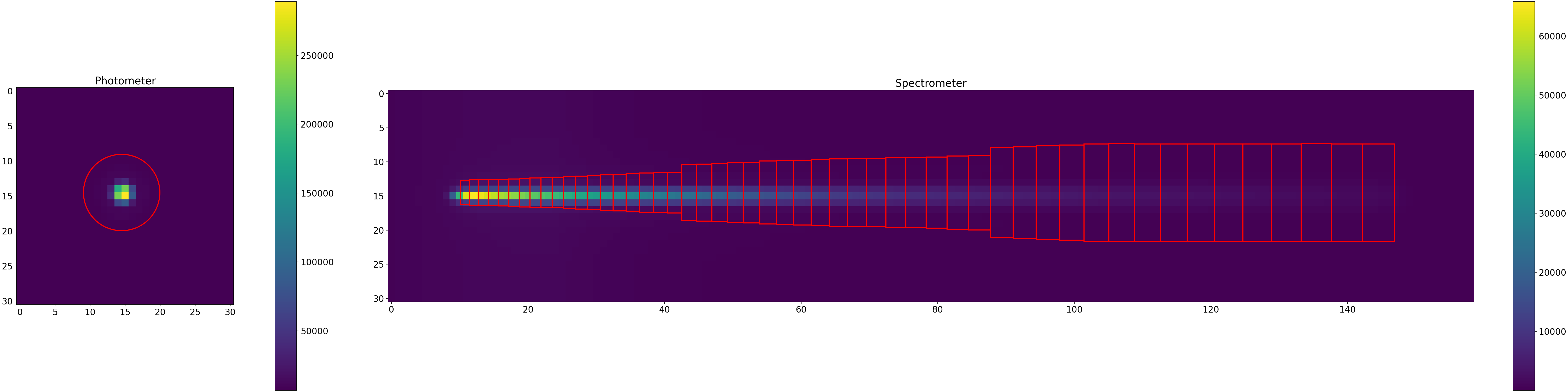
exosim-plot -i test_common.h5 -o plots/ --focal_plane -t 0
This will produce two plots: the first focal plane and the instrument efficiency vs wavelength:

Radiometric model#
Now you can run the radiometric model on top of the produced focal plane (see Radiometric Model):
exosim-radiometric -c main_example.xml -o test_common.h5
And, again, we can investigate the content by producing useful plots by
exosim-plot -i test_common.h5 -o plots/ --radiometric
This will plot the aperture used for the photometry
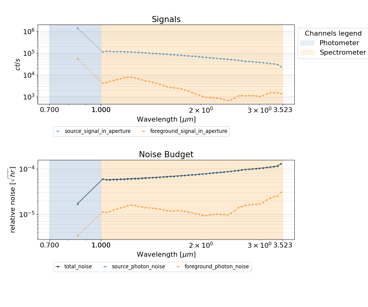
and the radiometric table
Sub-Exposure#
As for the radiometric model, on top of the produced focal plane we can build the Sub-Exposures (see Sub-Exposures):
exosim-sub-exposures -c main_example.xml -i test_common.h5 -o test_se.h5
And, again, we can use the dedicated plotter
exosim-plot -i test_se.h5 -o plots/ --subexposures
Which will produce an image of each Sub-Exposure for each channel and store it in the indicated folder
NDRs#
Finally, we can build the NDRs (see NDRS) on top of the Sub-Exposures:
exosim-ndrs -c main_example.xml -i test_se.h5 -o test_ndr.h5
And we can use the dedicated plotter
exosim-plot -i test_ndr.h5 -o plots/ --ndrs
Which will produce an image of each NDR for each channel and store it in the indicated folder.
From Python script#
Alternatively, a Python script is included which follows the previous steps: example_pipeline.py.
The content of the scripts can be summarised as
import exosim.recipes as recipes
from exosim.plots import RadiometricPlotter, FocalPlanePlotter, \
                        SubExposuresPlotter, NDRsPlotter

# create focal plane
recipes.CreateFocalPlane('main_example.xml',
                        './test_common.h5')
# run focal plane plotter
focalPlanePlotter = FocalPlanePlotter(input='./test_common.h5')
focalPlanePlotter.plot_focal_plane(time_step=0)
focalPlanePlotter.save_fig('plots/focal_plane.png')
focalPlanePlotter.plot_efficiency()
focalPlanePlotter.save_fig('plots/efficiency.png')

# run radiometric model
recipes.RadiometricModel('main_example.xml',
                        './test_common.h5')
# run radiometric plotter
radiometricPlotter = RadiometricPlotter(input='./test_common.h5')
radiometricPlotter.plot_table(contribs=False)
radiometricPlotter.save_fig('plots/radiometric.png')
radiometricPlotter.plot_apertures()
radiometricPlotter.save_fig('plots/apertures.png')

# create Sub-Exposures
recipes.CreateSubExposures(input_file='./test_common.h5',
                           output_file='./test_se.h5',
                           options_file='main_example.xml')
# run Sub-Exposures plotter
subExposuresPlotter = SubExposuresPlotter(input='./test_se.h5')
subExposuresPlotter.plot('plots/subexposures')

# create NDRs
recipes.CreateNDRs(input_file='./test_se.h5',
                  output_file='./test_ndr.h5',
                  options_file='main_example.xml')
# run NDRs plotter
ndrssPlotter = NDRsPlotter(input='./test_ndr.h5')
ndrssPlotter.plot('plots/ndrs')
From Jupyter notebook#
Finally, a Jupyter notebook is included containing the same scripts: example_pipeline.ipynb.
ExoSim Tools  #
#
ExoSim 2 includes a list of tools useful to help the user in preparing the simulation (see ExoSim Tools). An example script to run the tools is included (example_tools.py), which refers to the tools configuration file (tools_input_example.xml).