Signals#

The data flow in ExoSim is handled by the exosim.models.signal.Signal class. A signal behaves like an array, but with methods and arithmetic tailored to what the code needs.

The easiest way to see how it works is a simple case:

import numpy as np
from exosim.models.signal import Signal

wl = np.linspace(0.1, 1, 10) * u.um
data = np.ones((10, 1, 10))
time_grid = np.linspace(1, 5, 10) * u.hr

signal = Signal(spectral=wl, data=data, time=time_grid)

The signal variable now holds a Signal. The data is in the data attribute, and any units attached to it are in data_units.

The data is stored as a cube, as shown in the picture.

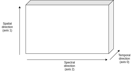
The grid along the spectral direction (axis 2) is in the spectral attribute, with its units in spectral_units. Likewise, the spatial grid (axis 1), if any, is in spatial with units in spatial_units, and the temporal grid (axis 0), if any, is in time with units in time_units. When a grid is not given, it defaults to \(0 \, \mu m\) for the spectral and spatial axes and \(0 \, hr\) for the temporal axis.

A dictionary of metadata can also be attached to a Signal.

data = np.ones((10, 1, 10))
metadata = {'test': True}
signal = Signal(data=data, metadata=metadata)

or they can be attached later as

data = np.ones((10, 1, 10))
signal = Signal(data=data)
metadata = {'test': True}
signal.metadata = metadata

In both cases

>>> print(signal.metadata)
{'test': True}

Units#

Units can be attached to the input data directly,

data = np.ones(10)*u.m
signal = Signal(data=data)

or passed separately:

data = np.ones(10)
signal = Signal(data=data, data_units=u.m)

The data can then be converted to other units:

signal.to(u.cm)

Derived classes#

Because units are supported, several specialised classes are derived from Signal:

exosim.models.signal.Sed, which has units of \(W \, m^{-2} \, \mu m^{-1}\)
exosim.models.signal.Radiance, which has units of \(W \, m^{-2} \, \mu m^{-1} \, sr^{-1}\)
exosim.models.signal.CountsPerSecond, which has units of \(counts \, s^{-1}\)
exosim.models.signal.Counts, which has units of \(counts\)
exosim.models.signal.Adu, which has units of \(adu\)
exosim.models.signal.Dimensionless, which has no units

You can initialise one of these classes directly to fix the data units. Otherwise, when units are attached to the data, the base Signal class picks the right derived class automatically.

Mathematical operations#

The Signal class and its derived classes support a set of mathematical operations. The examples below show the simplest cases, but the supported operations also include:

operations between Signal classes (as in the examples);
operations between a Signal and a numpy.ndarray or a Quantity;
operations in reversed order (array + Signal, not only Signal + array).

Units are carried through the operation. Multiplying a Dimensionless by a Sed gives a Sed, and so does multiplying a exosim.models.signal.Radiance by a solid angle. A Sed cannot be added to or subtracted from a Dimensionless. This holds between Signal classes and also between a Signal and a Quantity.

These operations also work on cached signals. See Cached signals for more.

Sum#

import numpy as np
import astropy.units as u
from exosim.models.signal import Signal

data = np.ones((3))
signal1 = Signal(data=data)

data = np.ones((3)) * 2
signal2 = Signal(data=data)

signal3 = signal1 + signal2

and hence

>>> print(signal3.data)
[[[3. 3. 3.]]]

Subtraction#

import numpy as np
import astropy.units as u
from exosim.models.signal import Signal

data = np.ones((3))
signal1 = Signal(data=data)

data = np.ones((3)) * 2
signal2 = Signal(data=data)

signal3 = signal1 - signal2

and hence

>>> print(signal3.data)
[[[-1. -1. -1.]]]

Multiplication#

import numpy as np
import astropy.units as u
from exosim.models.signal import Signal

data = np.ones((3))
signal1 = Signal(data=data)

data = np.ones((3)) * 2
signal2 = Signal(data=data)

signal3 = signal1 * signal2

and hence

>>> print(signal3.data)
[[[2. 2. 2.]]]

Division#

import numpy as np
import astropy.units as u
from exosim.models.signal import Signal

data = np.ones((3))
signal1 = Signal(data=data)

data = np.ones((3)) * 2
signal2 = Signal(data=data)

signal3 = signal1 / signal2

and hence

>>> print(signal3.data)
[[[0.5 0.5 0.5]]]

Floor division#

import numpy as np
import astropy.units as u
from exosim.models.signal import Signal

data = np.ones((3))
signal1 = Signal(data=data)

data = np.ones((3)) * 2
signal2 = Signal(data=data)

signal3 = signal1 // signal2

and hence

>>> print(signal3.data)
[[[0. 0. 0.]]]

Binning#

Two of the most useful methods on exosim.models.signal.Signal are the binning methods:

exosim.models.signal.Signal.spectral_rebin rebins the dataset along the spectral direction,
exosim.models.signal.Signal.temporal_rebin rebins it along the time direction.

Both are built on exosim.utils.binning.rebin, which resamples a function fp(xp) onto a new grid x, binning down where the new grid is coarser and interpolating where it is finer, but never extrapolating. It is optimised to resample multidimensional arrays along a given axis.

spectral_rebin and temporal_rebin are both documented with examples. Take spectral binning as an example. Start from the initial values:

>>> wavelength = np.linspace(0.1, 1, 10) * u.um
>>> data = np.ones((10, 1, 10))
>>> time_grid = np.linspace(1, 5, 10) * u.hr
>>> signal = Signal(spectral=wavelength, data=data, time=time_grid)
>>> print(signal.data.shape)
(10,1,10)

We can interpolate at a finer wavelength grid:

>>> new_wl = np.linspace(0.1, 1, 20) * u.um
>>> signal.spectral_rebin(new_wl)
>>> print(signal.data.shape)
(10,1,20)

or we can bin down to a new wavelength grid:

>>> signal = Signal(spectral=wavelength, data=data, time=time_grid)
>>> new_wl = np.linspace(0.1, 1, 5) * u.um
>>> signal.spectral_rebin(new_wl)
>>> print(signal.data.shape)
(10,1,5)

Writing, copying and converting#

A Signal also has methods to export its content.

It can be cast to a dict:

import numpy as np
from exosim.models.signal import Signal

data = np.ones((3))
signal = Signal(data=data)

dict(signal)

The result is a dictionary whose keys are the class attributes and whose values are their contents. Casting keeps only part of the exosim.models.signal.Signal information: the attributes data, time, spectral, spatial, metadata, data_units, time_units, spectral_units and spatial_units.

>>> print(dict(signal))
{'data': array([[[1., 1., 1.]]]),
 'time': array([0.]),
 'spectral': array([0.]),
 'spatial': array([0.]),
 'metadata': {},
 'data_units': '',
 'time_units': 'h',
 'spectral_units': 'um',
 'spatial_units': 'um'}

The exosim.models.signal.Signal.write method stores the content into an Output, most often an HDF5 file. For example:

import os
from exosim.output.hdf5.hdf5 import HDF5Output

output = os.path.join("output_test.h5")
with HDF5Output(output) as o:
    signal.write(o, "test_signal")

The output then holds the class information:

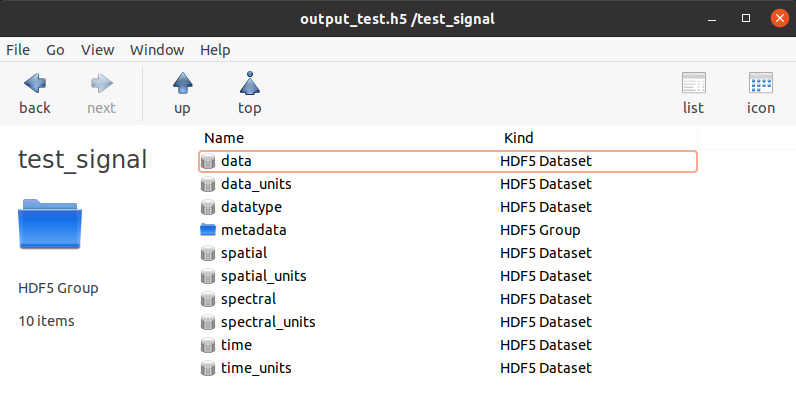
The stored information is the same as dict(signal).

The Signal class is also iterable:

>>> for k,v in signal1: print(k,v)
data [[[1. 1. 1.]]]
time [0.]
spectral [0.]
spatial [0.]
metadata {}
data_units
time_units h
spectral_units um
spatial_units um

Finally, a Signal can be copied with exosim.models.signal.Signal.copy:

copied_signal = signal.copy()

Cached signals#

A Signal can run in cached mode to handle very large datasets. The data then lives in a chunked h5py.Dataset, managed by CachedData. To create a cached signal, give it a HDF5OutputGroup or HDF5Output, the dataset shape and a dataset name:

import numpy as np
import astropy.units as u

from exosim.models.signal import Signal
from exosim.output import SetOutput

output = SetOutput('test_file.h5')
with output.use(append=True, cache=True) as out:
    cached_signal = Signal(spectral = np.arange(0,100) * u.um,
                            data=None,
                            shape=(1000,100,100),
                            cached=True, output=out,
                            dataset_name='cached_dataset')

The dataset is written to the file in chunks. Each chunk spans the full spectral and spatial shapes and as many time steps as fit in the chunk size, which defaults to 2 MB.

The chunk size is set through RunConfig, as described in Chunk size:

from exosim.utils import RunConfig

RunConfig.chunk_size = N

where N is the desired size of chunk in MB, which will be set for the environment.

If no output file is given, the code writes to a temporary file.

A cached signal is used slightly differently from a normal one. For a normal signal you read the datacube through the data attribute; for a cached signal you should use dataset instead. data forces the whole datacube into memory, which must be avoided for large datasets, whereas dataset is the chunked h5py.Dataset itself.

You can reach the chunks and set values with the h5py.Dataset methods. The example below iterates over the chunks and sets every value to 1:

for chunk in cached_signal.dataset.iter_chunks():
    dset = np.ones(cached_signal.dataset[chunk].shape)
    cached_signal.dataset[chunk] = dset

Otherwise, the data can be accessed as a normal NumPy array:

cached_signal.dataset[10,10,10] = 1

Note

A cached Signal can reach its h5py.Dataset only while the HDF5Output is open.

To make sure the edits land in the open file, flush them:

cached_signal.output.flush()

To loop over the chunks, ExoSim provides a dedicated helper, iterate_over_chunks:

for chunk in iterate_over_chunks(cached_signal.dataset,
                             desc="iterator description"):
    dset = np.ones(cached_signal.dataset[chunk].shape)
    cached_signal.dataset[chunk] = dset
    cached_signal.output.flush()