Focal plane#
Create focal planes#
The next step in the the Channel pipeline is to create an empty focal planet to populate.
This can be done with the method create_focal_planes
channel.create_focal_planes()
This method calls the CreateFocalPlane task.
This tasks, first build the focal plane array, by using CreateFocalPlaneArray.
Detector geometry#
The first step is the detector geometry that needs to be specified in the channel detector description:
<channel> channel_name

    <detector>
        <delta_pix unit="micron"> 18.0 </delta_pix>
        <spatial_pix>64</spatial_pix>
        <spectral_pix>364</spectral_pix>
        <oversampling>9</oversampling>
    </detector>

</channel>
In this case we are building a detector with 64 pixels in the spatial direction and 364 pixel in the dispersion direction, with pixel 18 micron wide. The oversampling key allows us to use sub-pixels. In this case we are splitting each pixel in 3 in each direction, hence having 9 sub-pixels.
Note
The main reason to have an oversampling factor is the jitter effect (see Instantaneous readout). The oversampling factor is needed to assure that the PSF is Nyquist sampled (at least 2 per FWHM) and to correctly represent intra-pixel response. The oversampling factor can be any number, but for efficiency reasons it should be a power of an odd value.
Wavelength solution#
If the channel is a spectrometer, then the wavelength solution is used to find the wavelength collected by each pixel in the dispersion. The solution can be specified as
<channel> channel_name
    <wl_solution>
        <wl_solution_task>LoadWavelengthSolution</wl_solution_task>
        <datafile>__ConfigPath__/wl_sol.ecsv</datafile>
        <center>auto</center>
    </wl_solution>
</channel>
The wl_sol.ecsv file is a table with 3 columns: Wavelength, x, y, where x is the dispersion direction and y is the spatial direction.
If y is set to 0 for each wavelength, the source light is assumed to be dispersed only along the dispersion direction, otherwise is to be dispersed also on the spatial direction.
The wavelength associated to each pixel in the spectral and spatial directions are stored along the focal plane in the Signal class in the spectral and spatial attributes..
The wl_solution_task indicates the task to use to load the wavelength solution.
By the default the LoadWavelengthSolution is used.
This Task can be customised, as described in Custom Tasks.
The center key is used to set the central pixel in the spectral direction. If “auto” it sets the central wavelength of the channel in the center of the pixel array. If a wavelength is indicated, it centers the wl solution on that wavelength. Else, it shifts the pixel array by the indicated number of pixels.
If the channel is a photometer there is no need to specify the wavelength solution.
The CreateFocalPlaneArray tasks will use the detector responsivity to estimate a wavelength solution to use for the next step (Rescale Contributions).
Source and foregrounds Focal planes#
Once the array is built, the CreateFocalPlane task creates a stack of array along the temporal direction.
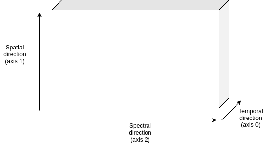
Finally, create_focal_planes duplicates it to produce a focal plane for the foreground contributions.
This method populates the focal_plane and frg_focal_plane attributes in the Channel class.
Rescale Contributions#
Knowing now the size of the focal planes and the wavelength solutions, we can rescale the incoming signal to convert them from signal densities (\(counts/s/\mu m\)) into proper signals (\(counts/s/pixel\))
channel.rescale_contributions()
The rescale_contributions method updates the sources and the path keys in the Channel class by rebinning the the signals according to the focal plane dispersion binning.
Then it estimates the wavelength solution gradient from the pixel wavelength solution and it multiply the signal by this gradient.
Populate focal plane#
Next it is finally time to populate the source focal plane. We now follow the following scheme:
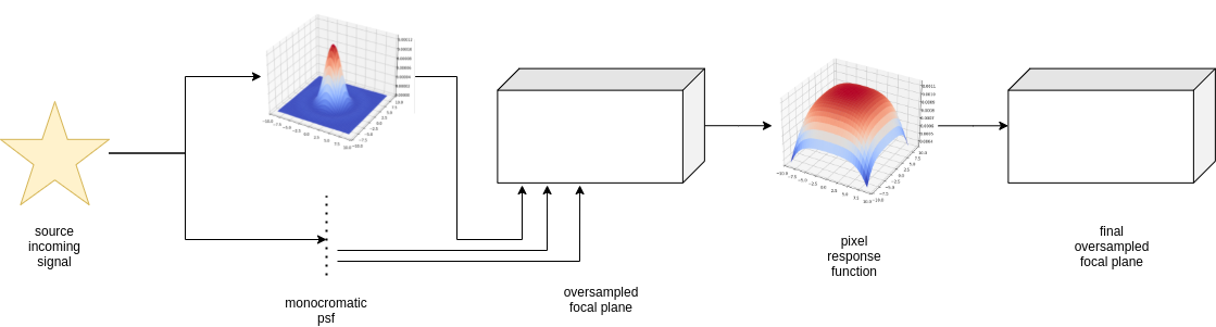
First we need to produce a monochromatic PSF for each wavelength sampled in the pixel wavelength solution. Then we multiply PSF by the source signal to the respective wavelength and we add the result on the relative pixel. On the now populated focal plane, we then apply the Intra-pixel Response Function (IRF).
The first steps are handled by
channel.populate_focal_plane()
The populate_focal_plane method calls PopulateFocalPlane task.
PSF#
The first step mentioned above is the production of the Point Spread Function ipercube.
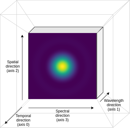
For each temporal step, the PSF cube is defined as in the following figure:
The PSF specifics are to be listed in the psf section of the .xml channel description. The simplest PSF are described by the Airy or by the Gauss functions.
<channel> channel_name
    <psf>
        <shape>Airy</shape>
    </psf>
</channel>
In this case, the PopulateFocalPlane task calls create_psf
This function produce a PSF cube as the one showed before, where the volume of ech PSF is normalised to unity:
The psf section can be customised by adding the following keys:
<channel> channel_name
    <psf>
        <shape>Airy</shape>
        <nzero> 8 </nzero>
        <size_y> 64 </size_y>
        <size_x> 64 </size_x>
    </psf>
</channel>
Where, nzero indicates the numbers of zero in the Airy function, size_x and size_y are the size of the PSF cube in the spectral and spatial directions. size_x and size_y can also be set to full to use the full size of the focal plane.
However, the user may want to load specific PSF shapes.
This can be done by writing a dedicated LoadPsf task.
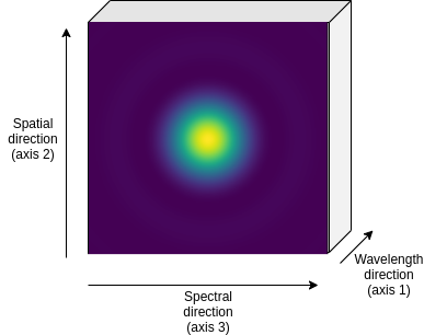
LoadPsf task produces an iper-cube, where to each temporal step of the focal plane is associated a PSF cube as the one in the previous picture.
The native PSF format supported by ExoSim is PAOS format and the functionality is provided by LoadPsfPaos.
In this case the user shall specify it in the .xml file as
<channel> channel_name
    <psf>
        <psf_task>LoadPsfPaos</psf_task>
        <filename>__ConfigPath__/paos_file.h5</filename>
    </psf>
</channel>
The LoadPsfPaos task loads the PSF cube provided by the filename data.
The PSF are then interpolated over a grid matching the one used to produce the focal planes, to convert them into the physical units.
Then the total volume of the interpolated PSF is rescaled to the total volume of the original one.
This allow to take into account for loss in the transmission due to the optical path.
The PSF are then interpolated over a wavelength grid matching the one used to for the focal plane, producing the cube.
This would fasten up the successive ExoSim steps.
The default LoadPsfPaos task does not include a temporal dependency,
and therefore the PSF cube is repeated on the temporal axis.
Note
For long observations with a small “low frequiencies variation” memory needed to keep the repeated PAOS Psf could be very high. It is possible to memorize and store only one PSF, switching to False the time_dependence parameter in the psf section, e.g.:
<channel> channel_name
    <psf>
        <psf_task>LoadPsfPaos</psf_task>
        <filename>__ConfigPath__/paos_file.h5</filename>
         <time_dependence>False</time_dependence>
    </psf>
</channel>
The user can define a temporal dependence by using a custom LoadPsf task.
An example using PAOS PSF is reported in LoadPsfPaosTimeInterp.
Finally, the PSF obtained are stored in the output file.
Adding PSF to the focal plane#
Once the PSF cube is ready, for each temporal step of the focal plane, we add a monochromatic PSF to the relative pixel multiplying it by the relative intensity of the source signal at the same temporal step. This allow us to produce a dispersed image in the case of a spectrometer or to cumulate the PSF in the case of a photometer. Also, if the source signal as a time dependent variation, this is propagated to the image on the focal plane thanks to the use of the same temporal step both in the focal plane and the source signal. The results will be an oversampled focal plane.
Intra-pixel Response Function#
The pixels on the focal plane do not have an uniform responsivity to the incoming light on their surfaces. They are known to be more responsive at the center and less to the edges. This effect can be represented in ExoSim introducing the IRF.
This is handled by the apply_irf method:
channel.apply_irf()
Create IRF#
The task to use to estimate the IRF is indicated as
<channel> channel_name
    <detector>
        <irf_task>CreateIntrapixelResponseFunction</irf_task>
    </detector>
</channel>
where CreateIntrapixelResponseFunction is the default class.
This tasks implements the equation presented in Barron et al., PASP, 119, 466-475, 2007 (https://doi.org/10.1086/517620).
It required the pixel diffusion length and the intra-pixel distance:
<channel> channel_name
    <detector>
        <irf_task>CreateIntrapixelResponseFunction</irf_task>
        <diffusion_length unit="micron">1.7</diffusion_length>
        <intra_pix_distance unit="micron">0.0</intra_pix_distance>
    </detector>
</channel>
Two other default tasks are available to create the IRF:
CreateOversampledIntrapixelResponseFunction.
The first one is a simple oversampling of the IRF, while the second one is a oversampling of the IRF with a larger size.
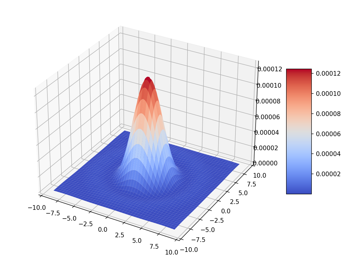
The user can however specify its own tasks and the relative parameters. Notice that the IRF volume is expected to be normalised to unity. Here is an example of a resulting IRF:
Caution
If no irf_task key is provided in the channel description,
the apply_irf method
automatically uses the default CreateIntrapixelResponseFunction task.
IRF application#
When the Pixel response function is produced, we apply it using the ApplyIntraPixelResponseFunction.
This task performs a convolution between the focal plane and the IRF.
Now the source focal plane is completed.
Note
In the default recipe (Focal plane automatic Recipe), if no irf_task key is provided in the channel description, the IRF step is skipped.
The user can specify the convolution method to use:
<channel> channel_name
    <detector>
        <convolution_method>fftconvolve</convolution_method>
    </detector>
</channel>
The available methods are: fftconvolve (scipy.signal.fftconvolve), convolve (scipy.signal.convolve), ndimage.convolve (scipy.ndimage.convolve) and fast_convolution (exosim.utils.convolution.fast_convolution).
If no convolution_method is specified, the default is fftconvolve.
Note
The fast_convolution method is the same implemented in Sarkar et al., 2021 <https://link.springer.com/article/10.1007/s10686-020-09690-9>`__. It is very accurate but it is slower than the other methods and requires a lot of memory. It is therefore recommended to use it only for small oversampling factor.
The CreateIntrapixelResponseFunction task creates a kernel compatible with both fftconvolve (scipy.signal.fftconvolve), convolve (scipy.signal.convolve) and ndimage.convolve (scipy.ndimage.convolve).
The tasks CreateOversampledIntrapixelResponseFunction is instead compatible with fast_convolution (exosim.utils.convolution.fast_convolution), which is a method developed specifically for ExoSim.
Populate foreground focal plane#
To populate the foregrounds focal plane, we can call the populate_foreground_focal_plane method:
channel.populate_foreground_focal_plane()
This involves the ForegroundsToFocalPlane task,
that simply adds the foregrounds contributions, stored in the path attribute, to the foreground focal planet, stored in the frg_focal_plane attribute.
If the path element to add is before a slit, the signal is dispersed. Therefore the contribution signal is convolved with a kernel of the width of the slit expressed as number of pixel, and then summed to the full array. If the slit width is expressed in number of pixel at the focal plane is \(L\), and the spectral resolving power computed at a certain \(\lambda_0\) is \(R(\lambda_0)\), the detector received diffuse radiation over the wavelength range \(\left( \lambda_j - \frac{L \lambda_0}{4 R(\lambda_0)} \, , \, \lambda_j + \frac{L \lambda_0}{4 R(\lambda_0)} \right)\), and not over the full range of wavelength accepted by the filter. So, the \(j\)-th pixel sampling the \(\lambda_j\) wavelength the collected signal is
If the path element to add is after a slit, or if no slit is in the path, the signal integrated on the full wavelength range is simply added to each pixel:
Now the foreground focal plane is completed.
Foreground sub focal planes#
If at least one optical element has
<optical_path>
    <opticalElement>
        ...
        <isolate> True <isolate>
    </opticalElement>
</optical_path>
Then the sub focal planes are computed. The same populate_foreground_focal_plane method also populates a frg_sub_focal_planes attribute.
This is a dictionary containing all the foreground signal contribution, highlighting the ones marked with isolate=True.
The sum of all the sub focal planes matches frg_focal_plane.
This mode allows the user to investigate the effects of a single optical surface.