Astronomical signals

Forewords

Now we can introduce some astronomical signals. Signals are intended as relative variations on the target source signal. So, they are defined as a function of the target source signal in time.

A few forewords before we start. Astronomical signals are not a core part of the ExoSim framework. ExoSim simulations are aimed at reproducing complex instrumental systematic effects. In order to train data reduction pipelines to cope with these effects, it is not necessary to introduce astronomical signals. Therefore, the astronomical signals we are introducing here are not intended as perfect representations of the expected ones, but only as representative, order-of-magnitude effects. For the same reason, we introduce them after the jitter, not before. Jitter is the most important effect to be reproduced, and it is also the most difficult to model. Introducing the astronomical signal before the jitter would make the jitter model more difficult to implement and the simulations significantly slower. This simulation order prevents ExoSim from simulating the spectral effect of jitter on the resulting signal, which is, however, a second-order effect compared to other noise sources.

This order-of-magnitude simulation of the astronomical signal is, however, improved compared to the previous version of ExoSim: this new version of the code also takes into account the smoothing effect on the astronomical signal caused by the instrument line shape and the intra-pixel response function. More details are reported in the following section.

Estimate the signal

The astronomical signals are intriduced in the sky configuration file, along with the source description. The Task describing the astronomical signal is called EstimateAstronomicalSignal. This is an abstract tasks with no model implemented. A complete example is reported in EstimatePlanetarySignal.

Here we report as example a signal that is the primary transit light curve of an exoplanet modelled using EstimatePlanetarySignal.

<source> HD 209458
   <source_type> planck </source_type>
   <R unit="R_sun"> 1.18 </R>
   <T unit="K"> 6086 </T>
   <D unit="pc"> 47 </D>

   <planet> b
      <signal_task>EstimatePlanetarySignal</signal_task>
      <t0 unit='hour'>4</t0>
      <period unit='day'>3.525</period>
      <sma>8.81</sma>
      <inc unit='deg'>86.71</inc>
      <w unit='deg'>0.0</w>
      <ecc>0.0</ecc>
      <rp> 0.12 </rp>
      <limb_darkening>linear</limb_darkening>
      <limb_darkening_coefficients>[0]</limb_darkening_coefficients>
   </planet>
</source>

In this example we point to EstimatePlanetarySignal task to model the primary transit light curve of an exoplanet thanks to the signal_task. Everything else under the planet tree is a parameter needed by the indicated Task. Note that planet is the keyword needed for EstimatePlanetarySignal, but it can be any other keyword, as long as the corresponding Task is able to parse it.

The user can define multiple astronomical signals for the same star. All of them are loaded and applied one at a time by ExoSim2.

Warning

The current version of ExoSim applies astronomical signals only to the target star. Please make sure to define the astronomical signal for the target star only. If astronomical signals are needed for multiple stars, multiple simulations can be defined, and the results can be combined later.

The astronomical signals are parsed by FindAstronomicalSignals, which looks for the signal_task keyword and instantiates the corresponding Task. The signal name is the parent tree keyword, in this case planet.

EstimatePlanetarySignal is based on the batman package presented in Kreidberg 2015. As usual, the User can replace the default Taks withg a custom one. The results of an EstimateAstronomicalSignal task shall be a 2D array with the first dimension being the wavelength and the second the time.

Warning

To run EstimatePlanetarySignal you need to have the batman package installed. Because the batman package is not a core dependency of ExoSim, it is not installed by default.

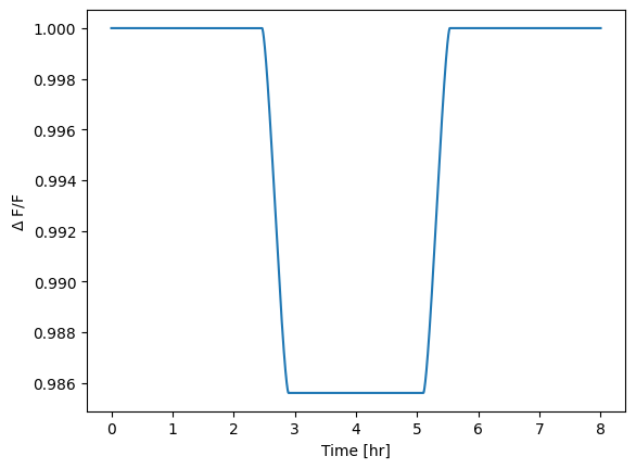
In this example the planetary radius is constantly 0.12 times the stellar radius, as indicated under the rp keyword. For a single wavelength, the transit light curve is the following:

If we want to simulate a transit with a varying radius, we can use the rp keyword to indicate a csv file.

<source> HD 209458
   <planet> b
      <rp> radius_data.csv </rp>
   </planet>
</source>

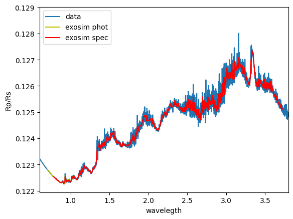
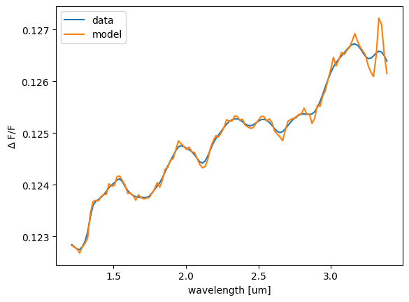
where the radius_data.csv file is a csv file with two columns, the first being the wavelength and the second the radius in stellar radii, entitled as rp/rs. In this case, the input data are binned by the Task. To give an example, we use a simulated forward model for HD 209458 b produced with TauREx3 and the resulting spectrum is the following:

The used file is available in the example/data folder of the ExoSim package.

Similarly, the user can define a wavelength dependent limb darkening using a csv file. In this case, the first column is the wavelength and the other columns are the limb darkening coefficients, entitled as ldc_c1, ldc_c2, etc.

Multiple signals can be listed in the sky configuration file, and they will be parsed and applied one per time.

Apply the signal

Instrument line shape

To apply the signal, the Instrument line shapes are needed. These are loaded from the focal plane file by the LoadILS task. The task returns a data cube of 1D PSFs for each wavelength. The data cube is a 3D array with the first dimension being time, the second wavelength, and the third the shape response in the spectral direction. These line shapes are normalised to their maximum value, so that the maximum value of the line shape is 1.

The instrument line shapes produced by this task are not the same as the instrument line shapes as defined in the literature. To be used as the instrument line shapes as defined in the literature, they need to be convolved with the intra-pixel response. This convolution is not part of this task, as it affects the way the ILS are sampled. The convolution with the intra-pixel response is done in the ApplyAstronomicalSignal Task, where the ILS are used to convolve the astronomical signal.

The LoadILS task is a default Task. If needed, it can be replaced with a custom Task.

<channel> channel_name
   <detector>
      <ils_task>LoadILS</ils_task>
   </detector>
</channel>

Signal application

Once parsed, the astronomical signal is applied to Sub-Exposures by the ApplyAstronomicalSignal task. This task convolves the astronomical signal with the instrument line shape and the intra-pixel response, weights the signal with the source flux on the channel (if provided), and multiplies it with the Sub-Exposures.

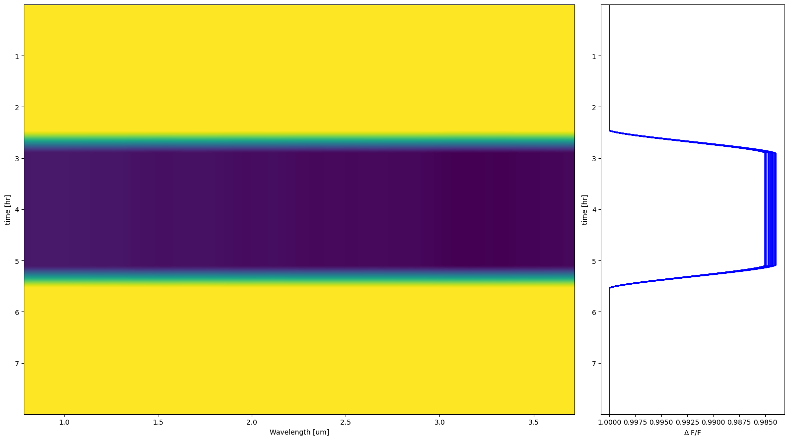
Here we show some example results. In the following, we are considering a spectrometer read using Correlated Double Sampling (CDS). We are considering a transit of HD 209458 b with a radius of 0.12 times the stellar radius. We select the second NDR for each ramp and divide it by the second NDR of the first ramp. Then we sum the resulting images along the spectral direction. The following picture shows the results. On the left panel, the transit light curve for each pixel is shown. So, the y-axis is time, while the x-axis is the pixel number, corresponding to a certain wavelength. On the right panel, the transit light curve for each wavelength is shown.

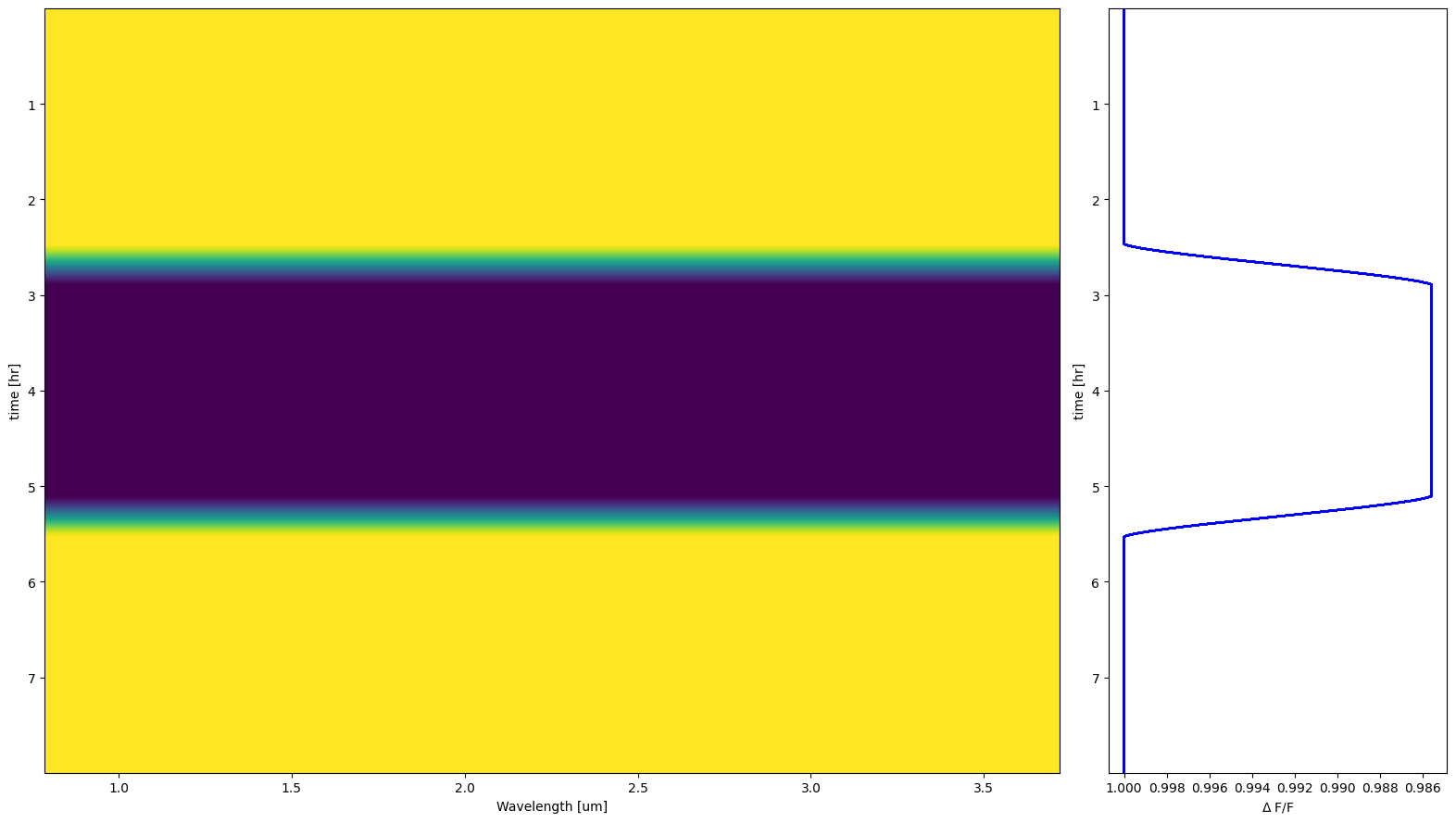
Because the transit depth is constant, the transit light curve for each spectral pixel is the same, and therefore the transit light curves on the right plot are aligned.

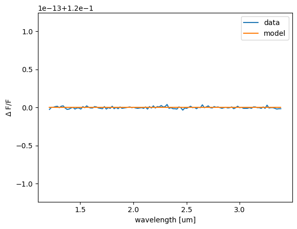
The following plot shows the transit depth at the centre of the transit for each wavelength. We compare the transit depth with the input model, which is the result of a constant radius ratio of 0.12 between planet and star, and we see that the two are the same up to the numerical precision of 1e-15.

In the following example, we use the same input parameters, but with a varying radius. The input model is the same as the one shown above for HD 209458 b. We can see now that in the first plot the transit light curves are no longer aligned.

Also, we compare again the transit depth at the centre of the transit for each wavelength with the expected model. We can see that the curve extracted from the ExoSim data is smoother than the input model. This is the effect of the applied ILS to the input model.