Reading Scheme#
Once the jitter time lines are ready, we need to define the reading scheme for the detector.
Note
In this model we are only considering instantaneous read out of the detector.
Assuming we want to reproduce the following reading scheme, which is the same of Sub-Exposures, where a \(60.3 \,s\) exposure time is sampled by 6 NDRs divided in 3 groups.
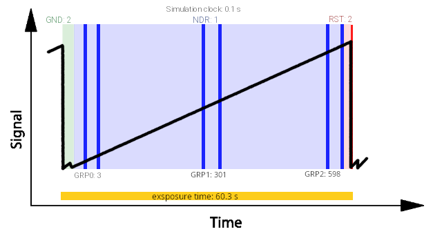
The ramp is sampled at the readout_frequency cadence, defined in :ref:sub-exposures creation. In this example, we assume:
Ground (GND) state lasts \(0.2\,s\), i.e. 2 simulation clocks at \(10\,Hz\);
The first NDR is read after 1 clock (\(0.1\,s\));
NDRs within a group are spaced by 1 clock;
Groups are spaced by 296 simulation clocks;
Reset (RST) state lasts 2 clocks (\(0.2\,s\)).
Given these parameters, the NDRs occur at the following clock indices:
First NDR: starts at clock 2 (after GND), ends at 3
Second NDR: starts at 4, ends at 5
Third NDR: starts at 300 (= 4 + 296), ends at 301
Fourth NDR: starts at 302, ends at 303
Fifth NDR: starts at 598 (= 302 + 296), ends at 599
Sixth NDR: starts at 600, ends at 601
Then the RST state completes the ramp at clocks 602–603
This amounts to a total of 603 simulation clocks at \(0.1\,s\) resolution, i.e. exactly \(60.3\,s.\)
<channel> channel name
    <readout>
        <readout_frequency unit="Hz">10</readout_frequency>
        <n_NRDs_per_group> 2 </n_NRDs_per_group>
        <n_groups> 3 </n_groups>
        <n_sim_clocks_Ground> 2 </n_sim_clocks_Ground>
        <n_sim_clocks_first_NDR> 1 </n_sim_clocks_first_NDR>
        <n_sim_clocks_Reset> 2 </n_sim_clocks_Reset>
        <n_sim_clocks_groups> 296 </n_sim_clocks_groups>
    </readout>
</channel>
The user can also set the readout_frequency in units of \(Hz\) instead of \(s\).
The reading scheme is computed by ComputeReadingScheme
import exosim.tasks.subexposures as subexposures
computeReadingScheme = subexposures.ComputeReadingScheme()
clock, base_mask, base_group_end, base_group_start, number_of_exposures = computeReadingScheme(
    parameters=parameters,
    main_parameters=main_parameters,
    focal_plane=focal_plane,
    frg_focal_plane=frg_focal_plane)
The outputs of this Task can be confusing, because is written to optimise the next step in the sub-exposures procedure.
In the following we discuss each of them.
clock: this is the simulation frequency, which is the inverse of high_frequencies_resolution defined in Sub-Exposures;base_mask: this is state machine for the reading operation on the ramp. In fact, a ramp is made of different states: ground state (GNS), reset state (RTS) and read states (NDR). This mask is a list of of 0 and 1, where 1 is for the steps indicating a read operation: Referring to the previous image, the base will look like [0, 1, 1, 1, 1, 1, 1, 0].frame_sequence: this is the full list of simulation stapes for each steps on the ramp repeated by the number of ramps. E.g. [2, 1, 1, 296, 1, 296, 1, 2].number_of_exposures: this is the number of exposures needed to sample the full observation using ramps of the exposure time size. To estimate this quantity, theTaskcompute the integration time usingComputeSaturation, which is why it need the focal planes.
The exposure time is computed from the configuration using a logic equivalent to hardware implementations (e.g. FPGA), counting clocks for each operation:
# define exposure time in seconds
exposure_time = (
    n_clk_GND                          # Ground state
    + n_clk_NDR0                       # First NDR
    + n_clk_NDR * (n_NRDs_per_group - 1)                    # Remaining NDRs in first group
    + (n_clk_GRP + n_clk_NDR * (n_NRDs_per_group - 1)) * (n_GRPs - 1)  # Other groups
    + n_clk_RST                        # Reset state
) * clock                              # Convert to seconds
This structure mirrors how readout operations would be sequenced in a detector control system or programmable logic, giving full transparency on timing and event spacing.
For testing reasons, because sampling the full observation can be long and produce a lot of sub-exposure, the user can force the number of exposure to use by
<channel> channel name
    <type> channel type </type>
    <readout>
        <n_exposures> 2 </n_exposures>
    </readout>
</channel>
Note
To help the user in defining the detector reading scheme, ExoSim include a dedicated tool: Readout Scheme Calculator.
The readout scheme along with all the information needed for the instantaneous readout
is computed by PrepareInstantaneousReadOut.